Adversarial Examples Demonstrate Memorization Properties

In this article, the last in the problem exploration section of the series, you'll explore adversarial machine learning - or how to trick a deep learning system.

Adversarial examples demonstrate a different way to look at deep learning memorization and generalization. They can show us how important the learned decision space and its properties are and how the training data and preprocessing affect that behavior. Adversarial examples demostrate similar properties to outliers in deep learning systems.

Prefer to learn by video? This post is summarized on Probably Private's YouTube.

You'll also explore how adversarial learning contributed to model growth with early approaches to adversarial training and robustness, and how today's approaches find correlations to memorization in diffusion models.

What is an adversarial example?

Adversarial examples are those which trick a machine learning model into behaving in unlikely or unwanted ways. You've probably seen some adversarial examples on social media or in the news, which are often referred to as "jailbreaking" if they attack a LLM system.¹ But the study of adversarial examples precedes the existence of LLMs, and can teach you about how deep learning models work.

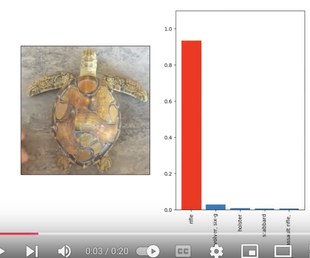
Let's examine an early example of an adversarial attack, from MIT researchers in 2017. The machine learning lab researchers were building on still image work that introduced adversarial examples by altering the images in small ways. They wondered if they could build a 3D adversarial example - and were able to do so!

Watch the full video on YouTube

Using then state-of-the-art computer vision models, they were able to 3D print an adversarial turtle which from many angles is improperly categorized as a rifle.

You might be wondering, how does that work???

How adversarial examples happen

Adversarial examples occur primarily by increasing uncertainty or error in the machine learning system. Via a variety of methods, adversarial examples push inputs into other areas of the decision space or boundaries (think about what you learned about margin theory!). In this case, the researchers wanted to push the turtle into "rifle" decision space. These attacks exploit those decision boundaries, in a similar way to how the training process creates them.

Let's walk through exactly how a simple adversarial attack works, to get an idea for how it happens.

You can take a model, really any model that is trained on a similar task -- here, a computer vision task. The properties of transfer learning make this possible. Deep learning models that are trained for similar tasks hold similar properties, learn similar things, and sometimes even have similar base datasets.

With your local computer vision model, you take an input that you want to make adversarial. Because you have direct model access, you can run the image through the model to produce an inference / prediction. When you do so, you can also observe the weights and activations at each layer, and of course the output of the inference. Let's say it correctly identifies a person in the image.

You want to make sure a person isn't found in the photo. You can then measure the gradient changes you would need to increase the error. You are essentially reversing the process of stochastic gradient descent, trying to increase error overall or towards another decision boundary (i.e. please make sure this photo has an imaginary boat in it). The goal is to reach an error level where the original classification no longer holds (i.e. the model returns that the photo has no person in it).

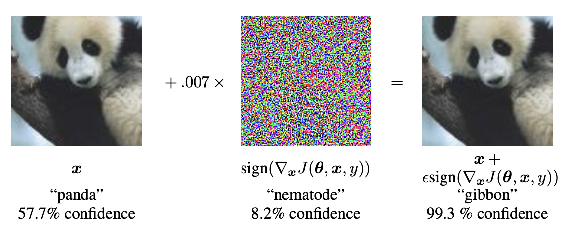
An example from one of the first well-cited papers on these attacks (Goodfellow et al, 2015) shows visually, what this might mean:

This attack uses the Fast Gradient Sign Method (FSGM), which functions similarly to what is described above.² This method shows you "which direction to push" and where in the input you should change to push that way. Then you actually create the perturbation, which aims to push the input in the right places in the right way, here: 0.07 (represented in the equation as e). This perturbation is combined with the original image, resulting in the large classification error (and resulting confidence in the incorrect gibbon class).

An attacker can use a method like this, or several more complex methods developed over time, to introduce error into model inference and influence the model to return a particular decision. The turtle becoming a rifle was a specific example to show deploying computer vision as security could go very wrong if you targeted people carrying "weapons".

In a way, these examples represent the unlikely inputs you see in the long tail of normal data collection. To a human, these are obvious, but to a computer vision or deep learning model, they are novel, erroneous or unknown. Interestingly enough, some of the initial defenses against adversarial attacks used this fact to correct the introduced error. Let's explore one of them that relates to our investigation of memorization.

Initial defenses: Manifold-ing

One of the early defenses that caught my eye had an interesting approach to the adversarial input problem. Instead of attempting to build the most robust model, it attempted to adjust the input and draw it closer to the more common examples, essentially regularizing the error away. This approach, called MagNet, was introduced by Meng and Chen in 2017.

Let's explore how this correction worked, step-by-step 😉:

1. First, potential adversarial examples are identified by a series of detectors. The detectors are trained to determine how abnormal the current example is based on the training examples. Numerous detectors were trained, so an adversary would need to know each of the detectors well enough to build an example that would 100% go through undetected³.

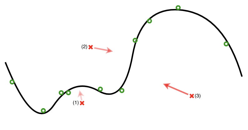
2. If an example is too far from the distribution of training examples, the images were corrected using an autoencoder built specifically to bring the example closer to the nearest training examples - here named a manifold. You can also think of this as attempting to migrate the examples closer to the nearest decision boundary, as you learned about in margin theory.

To visually illustrate an example of the output of this autoencoder, check out this diagram from the paper, which simplifies and visually explains the second step in 2-D. The curved line represents the manifold and the green circles the training examples. The red crosses represent adversarial examples, and the arrows represent their correction via the reformer.

1. Only then can the "reformed" version of the example be run through inference - hopefully without the carefully designed noise that would have disrupted the system without the correction.

This protection was successful against all of the common attack vectors at the time.⁴

How does this relate to memorization? Adversarial examples present the same types of problems for the network functionality as singletons, although they do so in different ways (one is malicious, the other just odd). If you treated singletons as adversarial, you could choose to focus on learning the nearest decision boundary or manifold and handling them as an outlier. This would reduce the chance of memorization.

In doing so, you might choose to implement something more like the reformer, which could assist in encoding information worth learning to shift decision boundaries but not enough to memorize the initial input. The reformer algorithm would be a stand-in for something like differential privacy, auto-encoding outliers towards a more "common" case. One approach that trains autoencoders as a way to encode privacy into a representation can be found in Dwork et al.'s work Fairness through Awareness.

These autoencoders and several other interesting approaches popular during those initial years were eventually replaced by a different approach to address adversarial examples.

The Heyday and Wane of Adversarial Research

Adversarial examples have likely existed as long as machine learning has existed, but they experienced a renaissance with deep learning due to the unique behavior of deep learning models in comparison to simpler models.

In 2016 it was hard to attend any machine learning event without hearing about adversarial examples (kind of like trying to avoid LLMs in 2024). There were dedicated sections of popular machine learning conferences just for papers and posters exploring these problems. These papers were looking at unique attack vectors, easy ways to produce adversarial examples and, of course, a variety of interesting and novel defense mechanisms, many of which were broken by other research sometimes days after publishing a new state-of-the-art defense paper.

Eventually newer approaches emerged -- ones that didn't try to figure out why or how adversarial examples worked or come up with clever ways to address them.

In 2018, a paper from MIT researchers (Mądry et al.) reached state-of-the-art adversarial performance with a new approach: throw compute and memory at the problem. Instead of trying to find, correct or otherwise disarm adversarial examples, they simply trained a bigger model for longer using adversarial examples alongside normal examples.

This works similar to the phenomenon you've been exploring in this series, where the double descent and increase in memorization enhances model performance. Instead of figuring out new and interesting ways to understand deep learning, you just memorize adversarial examples in a massive model and move along.

In addition to this approach, a second popular method came about when diffusion models rose in popularity. As you read about in a previous article, diffusion models can take an arbitrary noisy image and output prompt-based images. To do so, the diffusion process is reversed, so noise is gradually removed, shifting the output towards a known trajectory or goal. This can be applied to adversarial images in order to gradually remove potential noise.

Recent research on certifying adversarial robustness, a two-step process of applying a one-shot reverse diffusion process and then using a (probably fairly large) classifier achieved "state of the art" results. One interesting note is that a one-shot diffusion process works best, because iterative diffusers begin "filling in the blanks" and insert error by moving the input closer to an already learned class (or memorized input example). Choosing a less-diffused image results in higher integrity to the actual input. This demonstrates what you learned with regard to inpainting attacks.

Exploring the problem space

So far in this series you've learned about:

• how data is collected and labeled for machine learning
• how training and evaluation works
• why and how accuracy became the most important metric
• model size and training time growth
• what examples are memorized and some understanding and intuition on why and how
• how researchers first understood and found examples of memorization in deep learning
• how differential privacy relates to the memorization problems discovered in deep learning
• how adversarial examples demonstrate similar qualities as outliers
• how adversarial approaches influenced today's models and vice-versa

You now also know that memorization in deep learning happens. That it happens for common examples and outliers. That it's difficult to 100% understand and predict what is memorized. And that unless it is treated as a first-order problem which should be addressed and corrected, as adversarial examples were treated, memorization will continue to plague deep learning models. This memorization, as you have learned, presents serious problems to the privacy guarantees, and certainly to any person whose data is used for training.

In the next part of the article series, you'll explore the solution space. How can you address memorization? I'll walk you through active research areas, such as machine unlearning and differential privacy for training deep learning models. I'll also cover some areas which are useful but haven't gotten much attention, like personalized machine learning systems.

If you've enjoyed this series, consider subscribing to my newsletter. If you'd be interested in a printed version of this series, I'd love to hear from you. I hope to produce a zine (physical) version with artist illustrations and content modifications for ease of reading and based on reader feedback.

As always, I'm very open to feedback (positive, neutral or critical), questions (there are no stupid questions!) and creative re-use of this content. If you have any of those, please share it with me! This helps keep me inspired and writing. :)

Acknowledgements: I would like to thank Vicki Boykis for feedback, corrections and thoughts on this article. Any mistakes, typos, inaccuracies or controversial opinions are my own.