How Memorization Happens: Overparametrized Models

You've heard claims that we will "run out of data" to train AI systems. Why is that? In this article in the series on machine learning memorization you'll explore model size as a factor in memorization and the trend for bigger models as a general problem in machine learning.

To begin, what is meant by the word overparameterization?

What is a parameter?

In machine learning, a parameter is a value tied to the model's calculations. These calculations determine the model's predictions and how the model functions internally. You might have heard about parameter size, such as "this is the 7B (billion) parameter model" when using LLMs or other large generative models.

The parameters are set as the model is trained. Usually a parameter starts at a "random" state and is adjusted as part of the training process. The parameters updating creates the "learning" part of the machine learning training.

The parameter count also includes hyperparameters, with additional variables or inputs -- usually used by the training optimizers and learning algorithms. A hyperparameter is something a person can set beforehand, usually at a known state or range. Some hyperparameters can be adjusted as the model learns, such as setting an adaptive learning rate to expedite early stages of model training and then slow down with smaller steps as the model training enters later stages.

In a deep learning model, the most common parameters are weights and biases. Let's view a diagram to understand how these work:

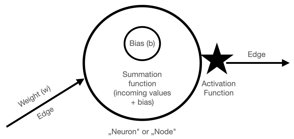
You can think of a deep learning model as a series of nodes, pictured above as a circle, and edges, pictured above as connecting arrows. The terms nodes and edges come from graph theory in mathematics, and you might know them from graph networks, like social network graphs.

In deep learning, the nodes here are the "neurons" and the edges connect neurons to one another. In this network, each input value can change the result of the equations in the node. Those equations within a node are calculated and each node sends the results over the edges to the next series of nodes, and so-on. This is why the original term "neural network" exists, since the nodes were compared to neurons.¹

In each node, there is a bias parameter which is part of the contained equation. The other values in the equation come from the incoming edges. Usually there are many nodes sitting at the same depth in the network. Together, these "same depth" nodes are called a layer.

Between each layer of nodes there are connections called edges. A weight parameter exists at the edges -- sitting "between" the layers. These weights connect each layer to the next layer. The number and type of connections can change with different types of deep learning architectures, but often there are at least a few fully connected layers which mean each node in one layer connects with an edge (and its accompanying weight) to the next layer of nodes.

When a data example is first encoded (see initial encodings article) and input into the model at the input layer, those input nodes calculate the result of their internal activation functions. Activation functions are usually calculated by taking the incoming values and summing the results with the node's biases and then running the result through a chosen activation function, which can vary by architecture. A common choice for an activation function today is ReLU because it has non-linear properties, allowing the network or model to learn more complex mathematics (alongside the power of linear algebra!).

The result of the activation function for a given node is transmitted as input to the next layer. This is calculated as inputs along the weight along the edge. This happens for each of the middle, hidden layers. In the final layer, the activations are condensed into a range of probabilities to make a prediction. This final step is heavily dependent on model type, architecture and the task at hand (i.e. generate text/image/video versus predict a class label).

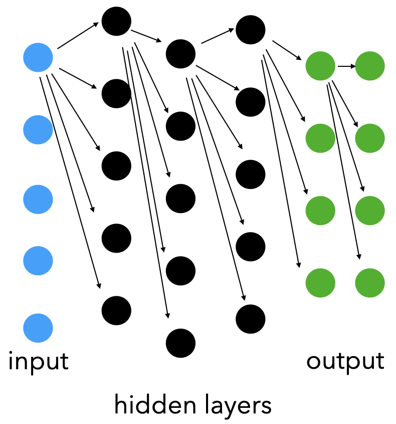Example of connected layers. Only the top nodes' edges for each layer are shown, but imagine this continues for every node in the model.

The training process updates the weights and biases, usually via some version of backpropagation, where error on whatever early guess the weights and biases have is transmitted backwards through the network. This error is used to update the parameters so the model can perform better on the next round of predictions. At a high level, this happens by reducing the weights, biases and resulting activations of the incorrectly identified guesses and increasing the weights, biases and resulting activations of the correct outcomes.

Now you have a high level understanding of parameters, let's investigate how they relate to model size.

Overparameterization and Model Size Growth

Since there must be at least as many parameters as nodes and edges, when the model's architecture grows and more layers are added, there will also be more parameters. In earlier deep learning, it was common to have between 100-200 layer models with a wide range of parameters per layer -- totaling between 20-120M parameters (see ResNet, VGGNet and AlexNet).

In today's deep learning, those numbers have exploded. Many deep learning models released since 2022 are overparameterized. This means they have more parameters than training data examples. If you've studied or used machine learning, you might be wondering if this results in overfitting. Overfitting is the ability for a model to exactly learn the training data, and therefore do poorly on unseen data. With overparameterized models, the model could potentially encode every example in the parameters.

The growth of model size and the subsequent growth of training time to ensure all parameters were adequately updated led to the discovery of double descent.

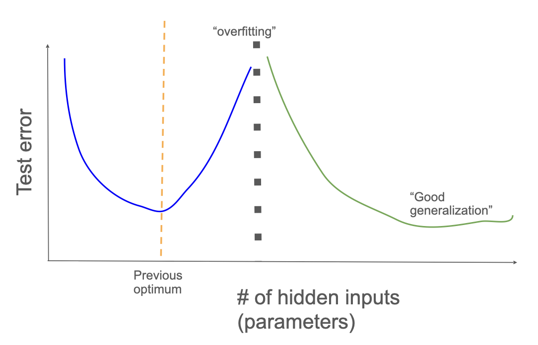
In smaller and older deep learning architectures, there was a point in parameter growth and training time where the model would overfit. This means that the model learned the training dataset too well (i.e. memorization and similar strategies) and therefore started performing poorly on the test dataset because of small divergences between the training and testing data.

As model parameters and training time increased, these larger models had a second descent of the error where the models generalized well and outperformed smaller models. This led to a massive investment in larger and larger models.

Tetko et al. studied overtraining as early as 1995. Overtraining increases the number of training epochs, and at that time this process created models that overfit and memorized the training dataset. That research recommended smaller networks with fewer hidden layers and less dense hidden layers, which could be trained without overfitting. They also recommended cross-validation via leave-one-out methods to compare models that had seen the data with those that hadn't (as you learned is a key part of memorization research).

When looking at how changes in layer size and depth over time -- they have grown massively since the 1990s. Just charting GPT parameter growth since the transformer architecture appeared (i.e. since 2018) is a good way to visually inspect the changes in parameter size.

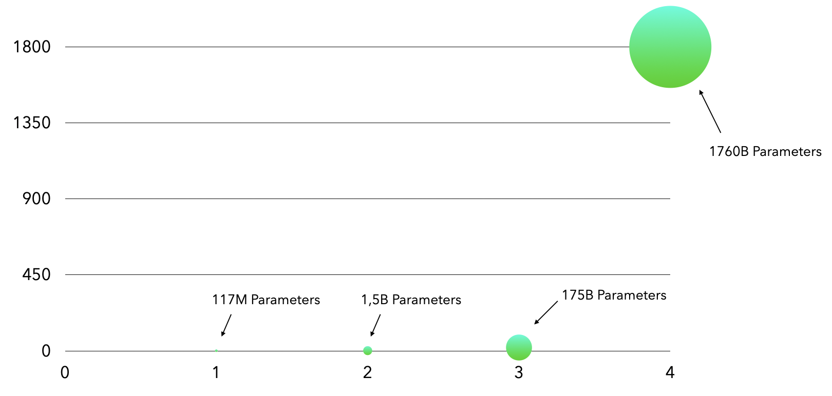
This chart looks at GPT parameter size based on what is known about the OpenAI GPT models. The first GPT was released in 2017 and had 117 million parameters. The second was released in 2019 and had 1.5 billion parameters, already a parameter growth of more than 12x. The third GPT came in 2020 and has 175 billion parameters (>100x size of GPT-2). Estimates of the GPT-4 put it at 1.7 trillion parameters, almost 10x bigger than GPT-3. As you can tell from this trend, there is a huge push towards ever larger models.

But understanding double descent and how deep learning works requires study. Simply embracing model size and training time growth without knowing how or what is changed by these aspects is unlikely to result in "forever" growth.² What, exactly, has changed in terms of models when they are overparameterized and trained for many more iterations?

Ummm, do we know how deep learning works?

This was the investigative question explored in the now famous paper Understanding Deep Learning Requires Rethinking Generalization (Chiyuan Zhang et al, 2017). You might remember Zhang's work from the last article, when he worked with Feldman on quantifying novel example memorization. Three years before that work, in 2017, the researchers were trying to understand exactly how computer vision deep learning models were learning with greater accuracy than before, especially with the increased architecture size.

They took the CIFAR10 and ImageNet datasets, then common datasets for large computer vision training and completely randomized the labels. Now the labels no longer applied to what was in the photo. A photo of a person was now a plane, a photo of a dog was now a building and so on.

Even with the labels completely randomized the training accuracy of the two most performant resulting models reached 89 percent. Of course, the accuracy on real data was awful, the model hadn't learned anything useful. But the fact that it learned completely random data opened new questions in understanding deep learning. This opened questions around common thinking about overfitting and generalization. How do we measure generalization? Do we understand the difference between memorization and overfitting?

The researchers called for more research and understanding of how memorization happens and a better understanding of what generalization is in deep learning. In larger models, generalization doesn't seem to behave the same way as generalization in smaller models -- in part due to the complexities of increasing parameter size and how that can leave enough parameters for both good generalization and memorization.

Learning the identity function

The identity function is a great example of a simple mathematical rule that could be trained using deep learning. The identity function takes an input and returns the input unchanged -- hence its name: identity. Think of it like adding 0 or multiplying by 1, but for more complex inputs.

Zhang et al. tested this idea in 2020 by training a few computer vision models to take in fairly simple input (the NIST and Fashion-NIST datasets) and learn the identity function.³ To investigate if the identity function could be learned versus just input memorization, they trained on just one training example repeatedly and altered the depth of the network (hence, the number of parameters).

They found that deeper networks with more parameters learned a constant function. What does that mean? Those networks learned to always answer with the example they were trained on, regardless of the input.

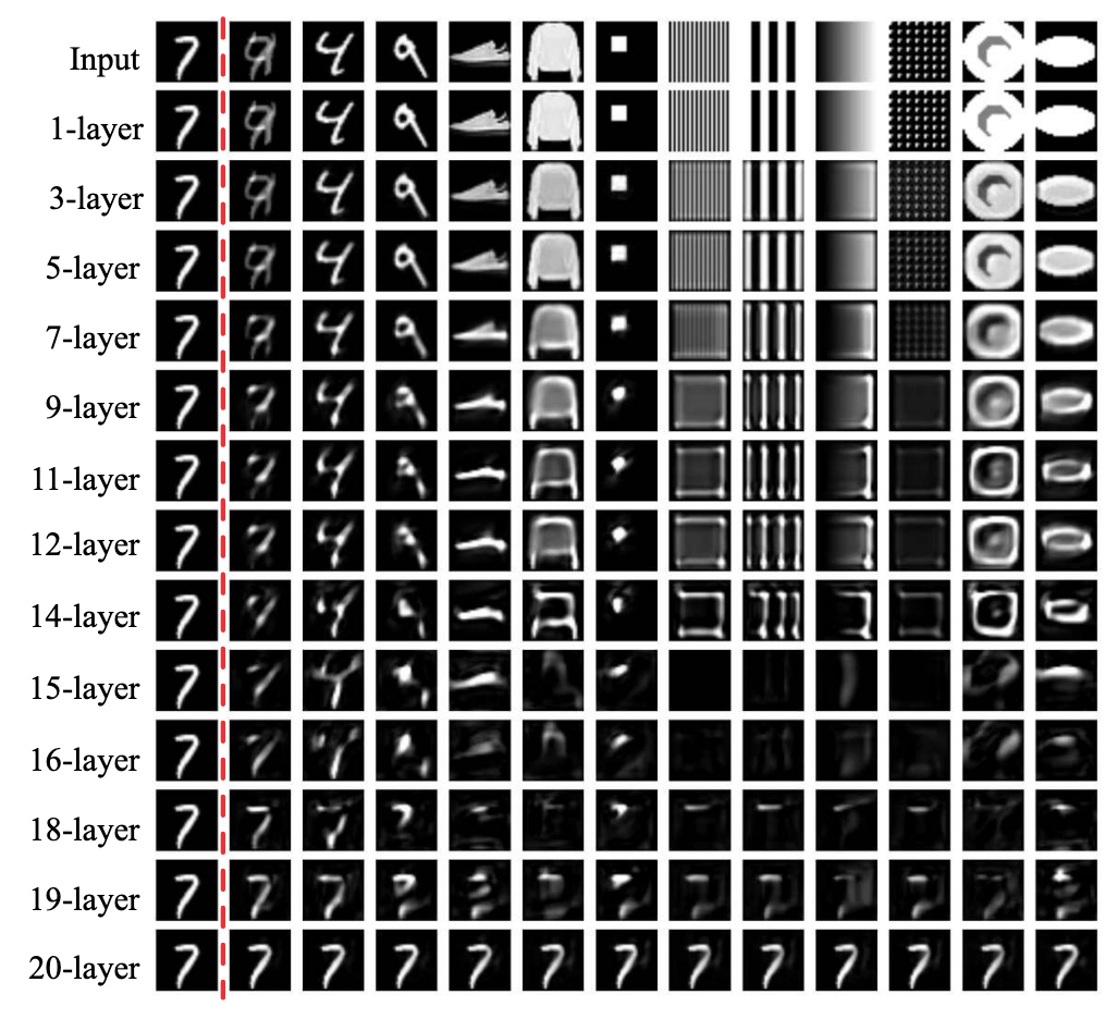Results of inference from CNN models trained with different depths. The 7 to the left is the entire training data for these models which attempted to learn the identity function. Each image is the prediction when given the input shown across the top row.

Intermediate depth networks learned to identify edges, which is probably a bit closer to the expected identity function (i.e. this is the outline of the shape you gave me), but not the same.

Very shallow networks sometimes learned the identity function (as shown in this example) but with other architectures or learning functions, they simply returned noise or a blank image.

Their conclusions were that computer vision models don't generalize the way that researchers and practitioners assumed they generalized -- and that more parameters might lead to more memorization instead of generalization.

But this research doesn't necessarily provide a better understanding of how to measure generalization. Related research from margin theory, however, did provide some insights!

Margin theory

Margins help estimate the generalization gap, or the difference between how a model performed during training and how it performs on unseen test data.

What is a margin? Margins are an important idea in support vector machines (SVMs), so let's use an example from SVMs to explain margins.

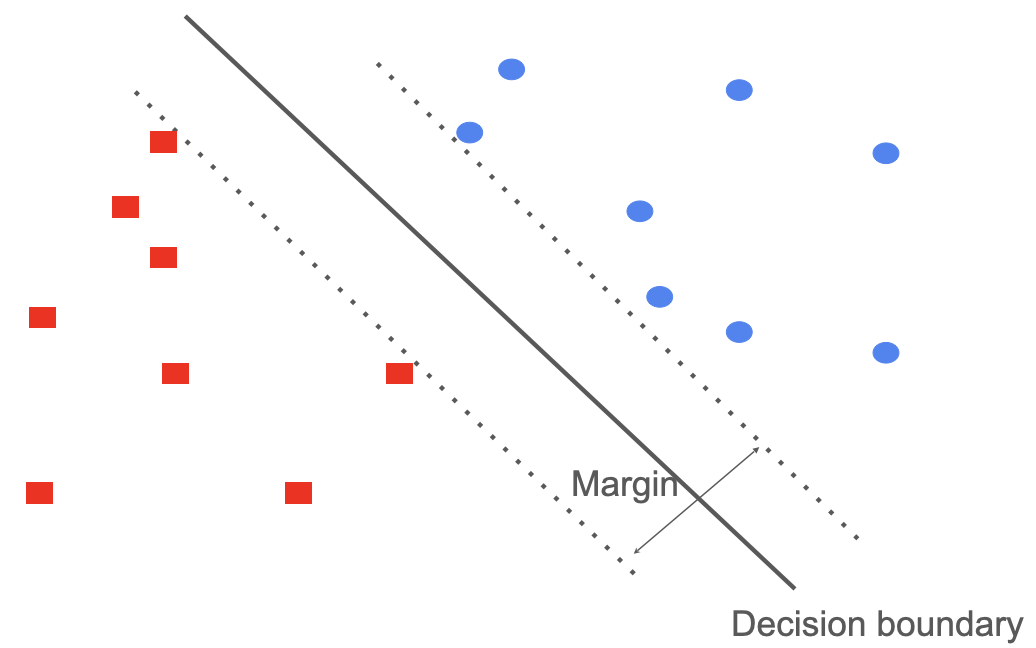
In support vector machines, you want to maximize the distance between the data points and the decision boundary. This improves the model confidence and avoids potential misclassification with "nearby" classes. Ideally, the boundary is further from the cluster of training examples, giving space to incorporate some "outliers", like the white peacocks.

But, how does this actually work in a high dimensional setting and with the complexity of a deep learning model? Deep learning models are more complex than support vector machines...

Research from Google has shown that margin theory applies if you take each layer of a deep learning model as its own decision engine. By sampling the distance between the intermediate input representation at that layer and the projected decision boundary, the margins can be estimated. The projected decision boundary is approximated via linearization even if the activation function is nonlinear.

To put it another way, you are sampling layers and approximating their decision boundaries against the current input. Measuring these margins and determining if the network is maximizing them, as with SVMs, provides an accurate prediction of the model generalization. The larger the approximated margins across several key layers, the better the performance on unseen data.

Google Research successfully built a new loss function to maximize margins while training deep learning models. The loss function penalizes predictions based on margin distance at different layers. The resulting models are more robust against adversarial attacks or other unintentional input perturbations. Neat that an idea from more simple machine learning, like SVMs, can also be useful in deep learning.

This provides some insight into memorization in large deep learning systems. Unlike SVMs, a deep learning model can create more decision boundaries due to its greater complexity and nonlinear learning. By memorizing outliers, a model can perform better on similar outliers that it sees later, even if these were not included in the original training data -- all because that outlier lands somewhere near the memorized input. This is one of the leading theories to explain why deep learning models memorize and generalize well.

In the next article, you'll look at how privacy research came to this conclusion about deep learning networks long before most machine learning research. You'll explore deep learning through the lens of differential privacy, a rigorous definition of to protect individual privacy.

I'm very open to feedback (positive, neutral or critical), questions (there are no stupid questions!) and creative re-use of this content. If you have any of those, please share it with me! This helps keep me inspired and writing. :)

Acknowledgements: I would like to thank Vicki Boykis, Damien Desfontaines and Yann Dupis for their feedback, corrections and thoughts on this series. Their input greatly contributed to improvements in my thinking and writing. Any mistakes, typos, inaccuracies or controversial opinions are my own.